Warwick iGEM computational modelling
Table of contents
Contents
Summary of project
The overuse of antibiotics has led to an artificial increase of selection pressure on bacteria. This has led to the rapid development of antibiotic resistant bacteria. Over the recent years, the number of antibiotic resistant strains has increased.
Wanting to aide in the arms race against such bacteria, we decided to pick a specific group of antibiotic resistant bacteria, and develop a technique to help reduce their threat.
Carbapenem resistant Enterobacteriaceae (CRE) also known as Carbapenem-producing Enterobacteriaceae (CPE) is a family of Gram-negative bacteria that are resistant to a class of antibiotics known as carbapenems which are only used to treat severe or high-risk infections. The current detection methods for it are: swabbing, which has a long turnover (sometimes up to four days); and Carba NP tests, which are faster but have a high false positive rates.
Our system was designed around CRISPR-mediated activation of the transcription of a fluorescent reporter. All the components were designed with in vitro usage in mind – which is why the operation of the system in a cell-free context should be possible without much work. The product would take the form of a tube with this cell-free solution which a sample, such as a swab, can be submerged into. A result would be visible under UV light in up to 30 minutes.

A photo of our finished detection kit
Custom modelling
To show that our proposed product would positively benefit the environment where it is proposed to be used, we wrote a custom stochastic computational model of the environment, with and without the product in use, and showed that when it is in use, the model scenario result improved.
We understand that computer models can become quite dry, particularly when explaining the details of their implementation. However, we believe that it is important to do this precisely, even at the cost of conciseness, as a small misunderstanding can be quickly amplified to an unexpected result, since the model’s high complexity causes it to have a chaotic output.
As a result of this, we created an in-browser interactive implementation of the model, which plots the output graph of the model based on the user inputting initial parameter states. We intend that this can quickly, intuitively, and interactively show the function and results of the model, which can help inform the goal throughout the implementation explanation, and provide a top-level understanding even if the rest of this page were omitted.
The whole project repository is available on GitHub, and the final production code for the project can be found: as a standalone Python file, or as a package on PyPI
Abstract
We designed and validated computational model of the spread of an antibiotic resistant pathogens in a hospital, with and without our diagnostic tool for quickly identifying it, and show that in a relevant scenario it reduces the presence of antibiotic resistant pathogens in our selected scenario, showing our product is beneficial in the real-world.
Summary of results
Our results show that our product will be beneficial in the real world. We know this as we validated our model to prove that it is a sufficiently close approximation to reality, then showed that the use of our product improved the model metrics, most notably the total number of deaths and the numbers of Carbapenem resistant bacteria across the run of a model.

Above shows a violin plot of the total number of deaths over a full run (i.e. till no people are infected) of the model with the validated parameters (discussed below). It is evident that the product causes a statistically significant reduction in the number of deaths resulting from the various strains of the pathogen modelled by the system.
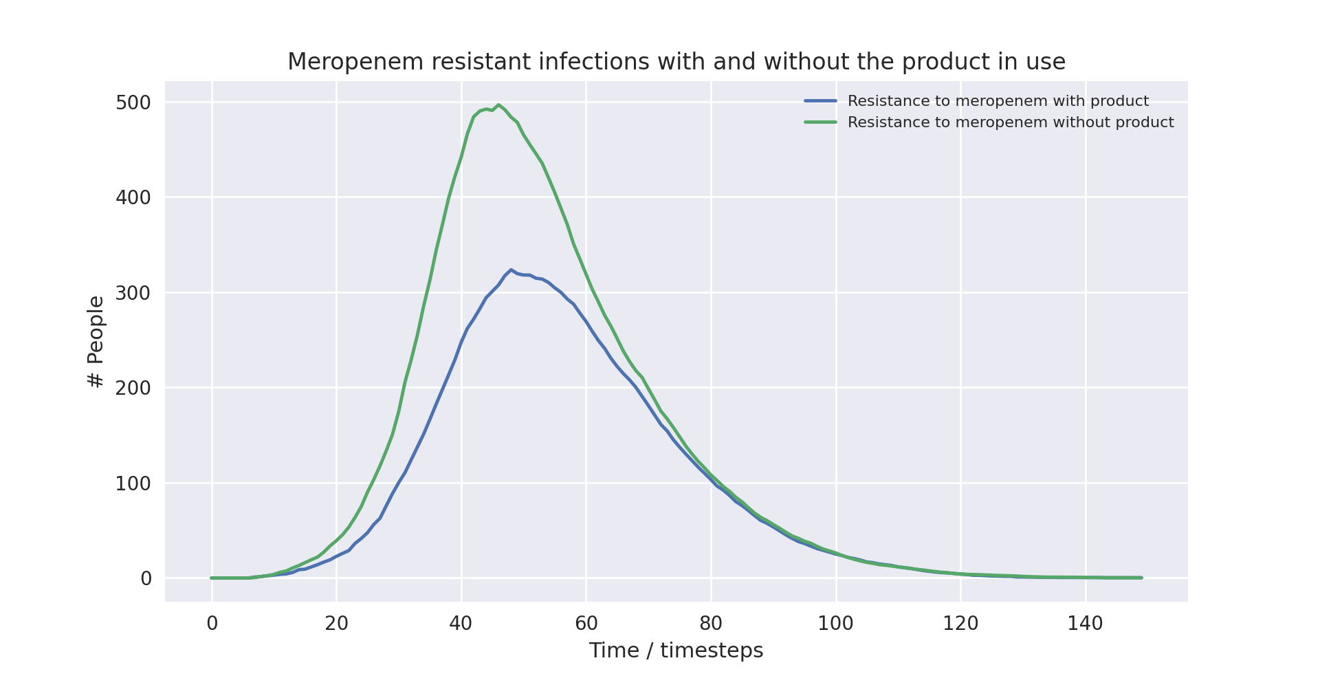
Above also shows a line plot of the total number of deaths over a full run (i.e. till no people are infected) of the model with the validated parameters (discussed below). It is again evident that the product causes a statistically significant reduction in the number of people infected with a strain of the pathogen resistant to meropenem - the drug resistance detect by our product.
Interactive web model
In order to demonstrate the model without requiring users to download the source code and its dependent libraries, then run it through python, we transpiled it into Javascript, so it can be run in the browser. This interactive transpiled model can be used below to demonstrate how parameters changes can affect the model outcome. Then, in the context section, we identify the parameters for the model which match it to the real world to show our product will work. In practice, having a model with interactive variables isn’t especially rigorous, but it does help show the power of the model, and how it can adapt to vastly different scenarios.
{{< model >}}
Model type
Our model is discrete time, stochastic, and compartmental:
Discrete time means that changes in the model occur at granular timesteps, like turns in a boards game
Below shows the code for how operations are performed on every person in the population each timestep, and data about them recorded
# Make a new data handler for each simulation
self.data_handler.__init__()

# Repeat the simulation for a set number of timesteps
for _ in range(NUM_TIMESTEPS):

    # For each person in the population
    for person in self.population:

        # Record the data throughout the model
        self.data_handler.record_person(person)
Stochastic means that the model is based on random probabilities, as opposed to a deterministic system of equations
A set of constant probabilities define the properties of the model
Transitions between states are chosen randomly with these constant probabilities
These probabilities, and other variable aspects of the model, such as population size or how many drugs are used, are set as constant values at the top of the model.
Initially, the model only had a parameter for how many different antibiotics are used, and all the associated probabilities (e.g. likelihood of recovery, likelihood of death, etc.) with these antibiotics were the same. However, in the final version, the different antibiotics are named to more closely map to the real world, and they are allowed to have their own separate values for these probabilities. However, for convenience’s sake, we introduce meta-parameters which can be used to set all the antibiotics to have the same probability in a given category.Below shows code for a default setting of these probabilities, the meaning of which will be explained further on:# General model parameters NUM_TIMESTEPS = 100 POPULATION_SIZE = 500 INITIALLY_INFECTED = 10 # Ordered list of drugs used, their properties, and the properties of their # resistant pathogens. Meropenem is a specific drug in the class of Carbapenems DRUG_NAMES = ["Amoxycillin+", "Meropenem", "Colistin"] PROBABILITY_MOVE_UP_TREATMENT = 0.2 TIMESTEPS_MOVE_UP_LAG_TIME = 5 ISOLATION_THRESHOLD = DRUG_NAMES.index("Colistin") PRODUCT_IN_USE = True PROBABILIY_PRODUCT_DETECT = 1 PRODUCT_DETECTION_LEVEL = DRUG_NAMES.index("Meropenem") ############################################################ # Use these if you want to set all drugs to the same thing # ############################################################ PROBABILITY_GENERAL_RECOVERY = 0 PROBABILITY_TREATMENT_RECOVERY = 0.3 PROBABILITY_MUTATION = 0.25 PROBABILITY_DEATH = 0.015 # Add time infected into consideration for death chance DEATH_FUNCTION = lambda p, t: round(min(0.001*t + p, 1), 4) PROBABILITY_SPREAD = 0.25 NUM_SPREAD_TO = 1 ########################################################################### # Set these explicitly for more granular control, or use the above to set # # them all as a group # ########################################################################### # Lookup table of drug properties by their names DRUG_PROPERTIES = {} DRUG_PROPERTIES["Amoxycillin+"] = ( PROBABILITY_TREATMENT_RECOVERY, ) DRUG_PROPERTIES["Meropenem"] = (PROBABILITY_TREATMENT_RECOVERY,) DRUG_PROPERTIES["Colistin"] = (PROBABILITY_TREATMENT_RECOVERY,) # Lookup table of resistance properties by their names NUM_RESISTANCES = len(DRUG_NAMES) RESISTANCE_PROPERTIES = {} RESISTANCE_PROPERTIES["None"] = (PROBABILITY_GENERAL_RECOVERY, PROBABILITY_MUTATION, PROBABILITY_SPREAD, NUM_SPREAD_TO, PROBABILITY_DEATH, DEATH_FUNCTION,) RESISTANCE_PROPERTIES["Amoxycillin+"] = (PROBABILITY_GENERAL_RECOVERY, PROBABILITY_MUTATION, PROBABILITY_SPREAD, NUM_SPREAD_TO, PROBABILITY_DEATH, DEATH_FUNCTION,) RESISTANCE_PROPERTIES["Meropenem"] = (PROBABILITY_GENERAL_RECOVERY, PROBABILITY_MUTATION, PROBABILITY_SPREAD, NUM_SPREAD_TO, PROBABILITY_DEATH, DEATH_FUNCTION,) RESISTANCE_PROPERTIES["Colistin"] = (PROBABILITY_GENERAL_RECOVERY, PROBABILITY_MUTATION, PROBABILITY_SPREAD, NUM_SPREAD_TO, PROBABILITY_DEATH, DEATH_FUNCTION,)
Additionally, there are internal settings, for example how the model outputs its results.
Compartmental means that the model is expressed in terms of the transitions between a set of states. The logic for these transitions forms a fundamental part of the model
Extensions from the SIR model
The model is at its core a modification of the standard “susceptible-infected-recovered” (often referred to as SIR) model for epidemic disease, which was first formulated in 1927 by Kermack and McKendrick [1].
This model can be described as three “compartments”, one for people susceptible to a pathogen, one for people infected with the pathogen, and one for those who have recovered from the pathogen.
People who are in the susceptible compartment can move into the infected when with a probability (\(\beta[S][I]\)) each time increment dependent on both the number of susceptible and number of infected people in the population.
People who are in the infected compartment can move into the recovered compartment each time increment with another probability \(\gamma[I]\).
Above shows a diagram of the SIR model transitions. Image source: [2]
From this, we can derive a set of differential equations which express the system, which is self-evident based on the above state transitions. Note that this is expressed as occurring of continuous time, however, this is just the limit of the time increments size going to zero.
We can then define a further metric \(\mathfrak{R}_0 = \frac{\beta}{\gamma}\), which is defined as the initial replacement number when one infectious individual is introduced into an all-susceptible population. This simplifies expressing the starting parameters of the model, which are themselves written as \([S]_0\), \([I]_0\), and \([R]_0\).

Above shows a graph of the SIR model over time. Image source: [2]
Our custom model extends this concept by adding more “compartments” for additional states people can take when they are infected with increasingly antibiotic resistant pathogens.
There are already examples of models of this extended class for examining antibiotic resistance in E. coli [3] [4] [5], showing that it is a suitable methodology for this problem. However, we believe that a custom model written from scratch was required to integrate the mechanism of the product being used.
Implementation
The key features of the model can be split up into its overall structure, and five distinct sections of its operation, which are enumerated in the sections below.
In each timestep of the model, each of these features are applied to change the state of the population. The order in which they are applied, whilst arbitrary, slightly affects the results of the model, in the sense that different application orders would give different results given the same random seed. We chose this order as we found during the validation section that it resulted in the closest fit to “reality”, by giving average results closest to real life data, but any application order can reasonably be considered an adequate model of the system. In our implementation, this order is:
FOR EACH person in the population
     Record the state of the person
     Increase treatment
     Isolate based on treatment level
     IF product is in use
             Isolate based on product
     ENDIF
     Recovery
     Mutation
     Death
ENDFOR
Spread through the population
1. Pathogen and people
A pathogen with a probability of death and a probability of recovery spreads through the population. The following statements taken from reality form part of the definition of our model:
Patients have a small chance of recovering by themselves, or can be treated with antibiotics, which have a larger chance of curing them
Different strains of the pathogen exist, which are resistant to different antibiotics
Pathogens can mutate to more resistant strains in specific circumstances explained in the mutation section
When they have recovered, they become immune to the all strains of the pathogen
Patients also have a small chance of dying due to the pathogen
Hence, patients can be in any of the disjoint states: uninfected, infected (possibly with resistance), immune, or dead.
In the limit of time to infinity, all individuals will be either uninfected, immune or dead, as they will all either not be infected in the first place, or recover or die from the pathogen.
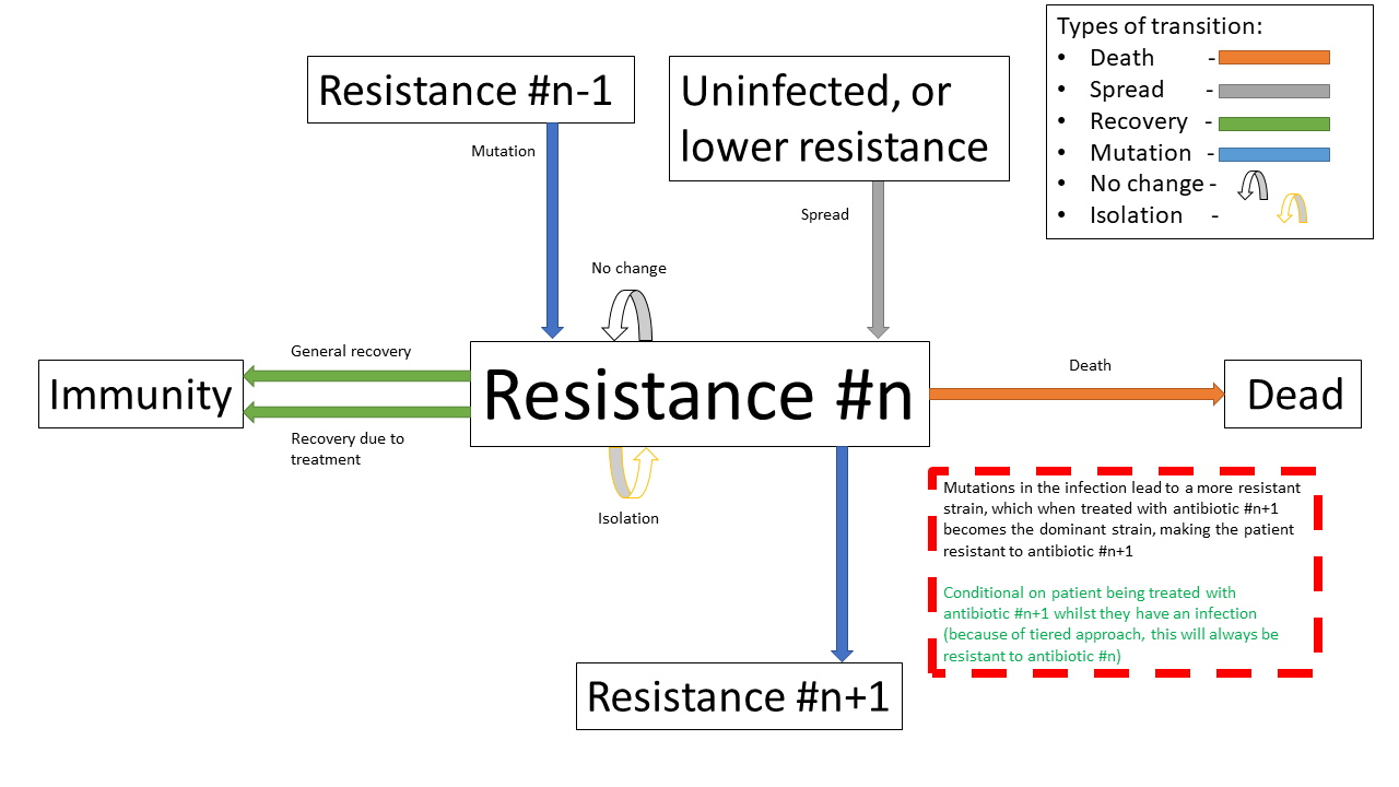
Below shows the state transition diagram of every state a person within the population can take (for reasons discussed later in the treatment section, pathogenic resistances to antibiotics will occur in a set order):

Below shows a state transition diagram of a person centred around the state of being infected with a pathogen resistant to antibiotic \(n\) in the precedence of antibiotics:

2. Treatment and mutation
Antibiotics are used in a specific order, which are numbered accordingly for clarity (with \(1\) being the first administered, and \(n\) being the last for antibiotics \(1..n\) ). This is to simulate the real-world, where different antibiotics are used in a tiered system, reserving the last for highly dangerous, multi-drug resistant pathogens - and is an important aspect of our model, as our product attempts to identify Carbapenem resistant Enterobacteriaceae (CRE), which are a type of these resistant pathogens.
Pathogens have a small chance of mutating to develop resistance to antibiotics being used to treat them, as such strains will only become dominant when there is a pressure giving them a survival advantage.
# Handle Mutation to higher resistance due to treatment
if decision(person.infection.mutation_probability):
    person.mutate_infection()
Below shows the same specified diagram used above, with additional information about the mutation step to elucidate it:
The pathogen is modelled as being immediately symptomatic, meaning doctors can immediately identify a patient is infected with it, but they cannot quickly identify whether or not they have a resistant strain if our product is not in use.
Once a person becomes infected, treatment with the lowest tier of antibiotics begins immediately, as they are immediately symptomatic.
If the pathogen is resistant to the antibiotic, the patient still has the opportunity to make a recovery on their own, but the antibiotic will have no effect. If the pathogen is not, the patient has the opportunity to recover both on their own, and via the antibiotic - increasing their likelihood of recovery each timestep.
Since multiple antibiotics are used in a tiered system, there must be a mechanism to move to a higher antibiotic.
There are a number of days which can be set as a parameter for the model, before which the same antibiotic will be used, then after this is exceeded a probability parameter is used each day to decide whether they will be moved up to a higher treatment tier.
Additionally, when our product is used and it detects a person to have a certain level of resistance, their treatment level is immediately increased to be above that resistance level, as we know that any other lower treatment will be ineffective.
# Handle increasing treatment
if person.treatment is None:
    # If the person is infected but are not being treated
    # with **anything**, start them on the lowest tier
    # treatment (we can know that the person is infected,
    # but not which tier they are on, without diagnostic
    # tools, as we can see they are sick)
    person.treatment = Treatment()
else:
    # If the person has been treated for a number of
    # consecutive days with the, a certain probability is
    # exceeded, move them up a treatment tier
    time_cond = person.treatment.time_treated > TIMESTEPS_MOVE_UP_LAG_TIME
    rand_cond = decision(PROBABILITY_MOVE_UP_TREATMENT)
    if time_cond and rand_cond:
        person.increase_treatment()

# Handle use of the product
if person.infection.get_tier() >= PRODUCT_DETECTION_LEVEL:
    if PRODUCT_IN_USE and decision(PROBABILIY_PRODUCT_DETECT):
        # If a person has the detected infection, put them on
        # a treatment course for it, (i.e. only ever change
        # it up to one above)
        if Params.DRUG_NAMES.index(person.treatment.drug) <= Params.PRODUCT_DETECTION_LEVEL:
            person.treatment = Treatment(Params.DRUG_NAMES[Params.PRODUCT_DETECTION_LEVEL+1])
3. Spread
Disease can spread from infected patients to uninfected patients, and patients with a less resistant strain. The likelihood of this occurring, and the number of people spread to each time can be controlled as parameters
# Spread the infection strains throughout the population
updated_population = deepcopy(self.population)
for person in self.population:
    if person.infection is not None and decision(PROBABILITY_SPREAD):
        for receiver in sample(updated_population, NUM_SPREAD_TO):
            person.spread_infection(receiver)
self.population = updated_population[:]
4. Isolation
Patients can be put into isolation, preventing the spreading the disease. This is the main place where the our product differentiates itself.
Without our product, a person is put in isolation when they exceed a threshold of treatment
With our product, since it provides a fast testing mechanism for highly resistant strains, patients can be detected as having the resistant strain, they are put into isolation when they exceed a threshold of having the resistant strain
# Isolate if in high enough treatment class (which
# is not the same as infection class - this will
# likely lag behind)
treatment_tier = Infection.get_tier_from_resistance(person.treatment.drug)
if treatment_tier >= ISOLATION_THRESHOLD:
    person.isolate()

# Handle use of the product
if person.infection.get_tier() >= PRODUCT_DETECTION_LEVEL:
    if PRODUCT_IN_USE and decision(PROBABILIY_PRODUCT_DETECT):
        # Put people into isolation if our product detects
        # them as being infected
        person.isolate()
Below shows the same specified diagram used above, with additional information about the isolation step to elucidate it:

5. Recovery and death
As discussed in section (1), each timestep, patients can recover (either naturally or via treatment), or patients can die.
Recovery makes the patients immune, meaning they cannot be infected again, essentially removing them from the system. Death also removes patients from the system.
# Handle Recovery generally or by treatment if currently infected
general_recovery = decision(person.infection.general_recovery_probability)
treatment_recovery = (person.correct_treatment() and
                    decision(person.treatment.treatment_recovery_probability))
if general_recovery or treatment_recovery:
    person.recover_from_infection()
    # Don't do anything else, as infection/treatment will
    # now be set to None
    continue

# Handle deaths due to infection
death_probability = person.infection.death_function(
    person.infection.death_probability,
    person.time_infected
)
if decision(death_probability):
    person.die()
    # Don't do anything else, as infection/treatment will
    # now be set to None
    continue
The goal is to create a situation where in the limit of time, the number of uninfected and immune people is maximised, and the number of dead people is minimised.
Software engineering
Model design process
We used an iterative design process during the development of the model, as discussed on page 21 in the book “Testing and Validation of Computer Simulation Models: Principles, Methods and Applications” [6].

Above shows a block diagram of steps in model design - taken from “Testing and Validation of Computer Simulation Models: Principles, Methods and Applications” [6]
We went through three iterative design stages of increasing complexity and proximity to real life before settling on our production code:
The first version was a very simple Markov model of people who could be infected forming a population. It did not employ the tiered system of antibiotic treatments, so did not map very closely to the real world. The code is available here
The second version was an improvement on the first in terms of mapping closer to reality by employing the tiered system of antibiotic treatments. It did this by adding additional
InfectionandTreatmentclasses as properties of aPerson, and additional logic to move “upwards” across them in a specific order. The code is available hereThe third version had a number of additional, but smaller, improvements with respect to closely modelling reality. There was an addition of a lag time before people could move up treatment, and the feature that the change of death increases over time being infected. The code is available here
The final production version included a fairly holistic re-write, in order to add finer granularity of control through parameters, allowing different infections to have different properties, and other additional parameters. On top of this, the version was rigorously tested by hand and via automated tests to identify conceptual errors. The code is available as the main production code on GitHub and PyPI
Note that none of these development code files have been rigorously tested in the way the final version has, so are likely to contain conceptual, or even syntax errors. The only purpose of providing access to them is to show the process of development, not to provide them as working models.
Automated testing
Whilst testing strategies and reasoning for testing are discussed in the
“Testing and validation” section, the implementation of the testing is a
point of interest in its own right. We used the unittest module in
Python to implement tests for the source code.
An example of a test is as follows, where we check that the boundary case of no-one being infected to start results in no infections for the entire model one. Whilst this might seem trivial, if it fails it is clear something is very wrong with the model, which might be a subtle result of a change made during development, and hence can prevent confusion about model results not making sense by showing that the problem is in the model implementation, not the analysis.
class TestModel(unittest.TestCase):
    def test_empty_model(self):
        """Test that a model with no infected people always stays fully uninfected"""
        # Change parameters for the test setup and run the test
        Params.INITIALLY_INFECTED = 0
        m = run()
        self.assertEqual(m.data_handler.get_uninfected_data(),
                         [Params.POPULATION_SIZE]*Params.NUM_TIMESTEPS)
        self.assertEqual(m.data_handler.get_infected_data()[0],
                         [0]*Params.NUM_TIMESTEPS)
        reset_params()
An interesting note about these tests is despite the fact they are written as unit tests, which normally refers to tests with a fixed input, these can be thought of as being tested with different inputs dependent on the result of the random number generator.
class TestModel(unittest.TestCase):
    def test_empty_model(self):
        """Test that a model with no infected people always stays fully uninfected"""
        # Change parameters for the test setup and run the test
        Params.INITIALLY_INFECTED = 0

        # Repeat the testing phase many times, with random number generation as the
        # function input differing each time
        for _ in range(100):
            m = run()
            self.assertEqual(m.data_handler.get_uninfected_data(),
                             [Params.POPULATION_SIZE]*Params.NUM_TIMESTEPS)
            self.assertEqual(m.data_handler.get_infected_data()[0],
                             [0]*Params.NUM_TIMESTEPS)

        reset_params()
If the tests are run many times, with many different resulting random number inputs, these unit tests can now be thought of as property based tests. This refers to checking that a function fulfils a property by randomly providing it with values from its input domain, and checking that the resultant outputs fulfil the property. This is a strategy which was pioneered in the functional programming language Haskell [7], and is often considered preferable to unit based tests [8].
The whole set of property based tests we wrote can then be run using the
pytest command:

Version control and CI/CD
Having implemented a robust testing strategy, we now had all the building blocks for a continuous integration/continuous development workflow, as shown below:

The build phase is relatively simple - writing the code in an editor of your choice, and running it with the Python interpreter, and the testing phase is discussed above.
Throughout the entire project, we used git as version control. From
this, we linked the project to a remote repository on GitHub, which is
the main way to access the most up to data code, so forms both the merge
and continuous delivery steps. When code is pushed to the remote
repository, actions are automatically run to ensure that the code is
both syntactically and conceptually correct, using the static analysis
tool flake8 for the former,
and by running pytest on all the code as discussed above for the
latter.
We chose not to automate publishing the code to PyPI (discussed below), which could be considered the production aspect of the modelling, as the project was under active development, and minor changes to the repository should not necessarily be pushed - as their general stability and usefulness is not fully known.
Transpilation to Javascript
In order to create the web-based version of the model, we needed to use a language which can be run client side in the browser. Since Python cannot do this, we needed to convert the source code into a language which can - with the obvious choice being Javascript, due to its ubiquitous use in this environment.
Instead of manually re-writing the entire model into Javascript, we decided to use an automated tool to do it for us. This class of tool is called a transpiler, which converts between two languages in the same tier in the language complexity hierarchy (e.g. two high level languages). We considered a number of tools, with the main decision being between Brython, a runtime transpiler which translates the Python code to Javascript on the fly, and Transcrypt, a build-time transpiler which translates the code beforehand. We decided to use Transcrypt, as it offers better performance, having pre-compiled the code, and since it allows an easier integration into the Javascript DOM.
The transpilation process was not totally seamless, as some language
properties in Python are not supported in Javascript, for example named
parameters and adding lists, and not all of the libraries used were
supported by Transcrypt, meaning some of the random methods had to
be re-implemented within the source code, and the output graphs and
excel exporter functionality had to be removed.
In order to display the output in a visual manner, we used the Chart.js package, which is commonly used for client side data plotting.
Uploading to PyPI
Since we developed our model in python, we uploaded it to PyPI, the Python package index. We did this as it greatly simplifies the way in which the package can be distributed. Instead of cloning the repository, and running the code directly through that:
git clone https://github.com/EdmundGoodman/Warwick_modelling
cd modelling/tiered-antibiotic-resistance-model
python3 model.py
The module can be installed using pip on the command line, then just
imported directly in a Python file:
pip install tiered-antibiotic-resistance-model
from tiered_antibiotic_resistance_model import *
run_and_output()
Furthermore the parameters of the model can be set within the other
Python file by directly manipulating the Param object, instead of
having to go into the source code and change them in the actual model,
which is not a best practice.
Testing and validation
It is important to remember that computer models are not infallible. It is impossible for a computer model of a system to “perfectly” emulate the real system, as that would require total simulation of the entire universe, which is evidently unfeasible. However, closely approximate models provide a wealth of information when correctly implemented, and can provide a level of abstraction to make the applicable in a wide variety of cases.
To ensure that models are sufficiently accurate to the real-world scenario they are trying to emulate - which is required for us to use them to draw conclusions about whether our product will be beneficial, it is important to test and validate them.
Levels of validation
In the paper “Validating Computational Models” by Kathleen Carley [9], there are four levels of validation described for computational models:
1. Grounding
The paper defines the grounding technique in the following ways:
“Grounding involves establishing the reasonableness of a computational model” [9]
“Grounding involved the use of story-telling, initialization, and evaluation techniques” [9]
Story-telling: “The basic goal of grounding is to establish that the simplifications made in designing the model do not seriously detract from its credibility and the likelihood that it will provide important insights” [9]
Initialization: “On the initialization front, grounding requires setting the various parameters and procedures so that they match real data” [9], for example comparing model outputs, and trends
Performance evaluation: “Simple performance evaluation is the process of determining whether the computational model generates the stylized results or behavior expected of the underlying processes” [9]
For “story-telling”, the above explanation of the implementation explains the mapping of the model to the real world. The variables within the model are named clearly so the “story” of the model can be inferred directly from the source code. Both initialization and performance evaluation are encompassed by the following sections on calibrating and verification.
2. Calibrating
The paper defines the calibrating technique in the following way:
“Calibrating is the process of tuning a model to fit detailed real data. This is a multi-step, often iterative, process in which the model’s processes are altered so that the model’s predictions come to fit, with reasonable tolerance, a set of detailed real data. This approach is generally used for establishing the feasibility of the computational model; i.e., for showing that it is possible for the model to generate results that match the real data. […]
Calibrating a model may require the researcher to both set and reset parameters and to alter the fundamental programming, procedures, algorithms, or rules in the computational model. Calibrating establishes, to an extent the validity of the internal workings of the model and its results (at least in a single case).” [9]
We inherently used calibration throughout the development phase of the project (see diagram in software engineering above), as the design process involved iteratively designing models, testing them on the scenario data we selected, and adding features and fixes to improve the resemblance of the model to “real life”.
3. Verification
The paper defines the verification technique in the following way: “Verification is a set of techniques for determining the validity of a computational model’s predictions relative to a set of real data. To verify a model, the model’s predictions are compared graphically or statistically with the real data” [10]
We graphically compared the data outputs with the expected characteristic “S-curve” shape which is prevalent in SIR type stochastic models similar to ours. Whilst the individual lines for different resistance levels do not form such a curve, if their total is taken, it does - which is the expected behaviour, as the sum of the resistance levels gives total number infected.
This is shown below with the boundary between the light and dark blue items in the graph forming the characteristic curve, which matches the shape of the light blue line in the SIR explanation graph.
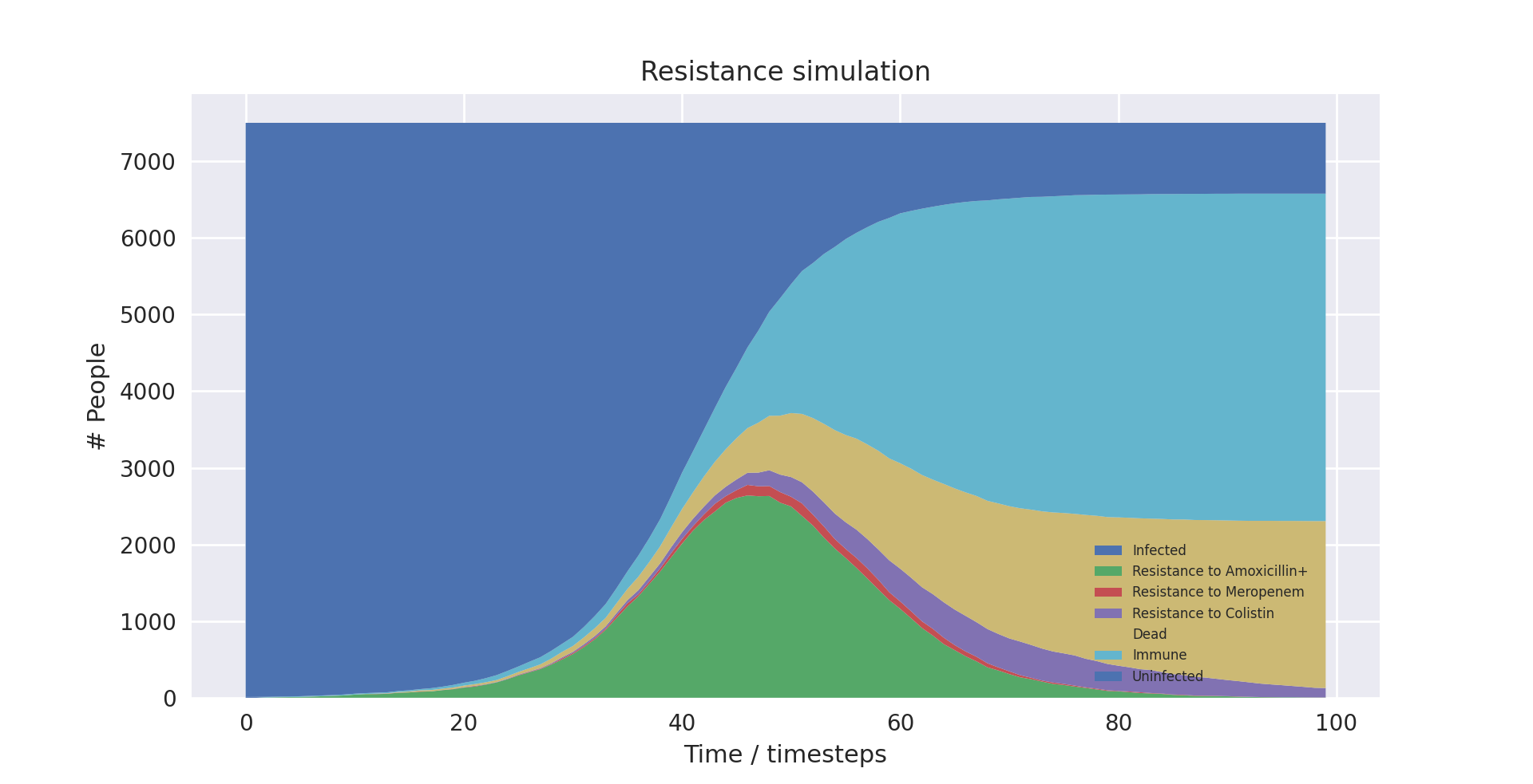
Above shows a stack plot of our model output showing the characteristic ‘S-curve’ shape
Above shows a graph of the SIR model over time - with the blue line being the same shape as seen in the above stackplot output of our model. Image source: [2]
Additionally, the book notes that “A special issue in verification occurs with respect to multi-agent models. Multi-agent models can potentially undergo dual level verification; i.e., verification at both the individual and group level. To wit, does the model accurately predict group level behavior, individual level behavior, or both?” [9]
Since our model can be considered to be multi-agent, as it is composed
of multiple Person classes forming a population, we needed to take
account of this special issue.
4. Harmonization
Harmonization is the final, and most complicated, stage of validation proposed in the book. It involves taking multiple sets of data for verification, then forming a linear model from them, and comparing the computational model the the linear one. Given the below reasons, we did not research what forming a linear model of the data entails.
We did not attempt harmonization on our model as we thought it was out of scope. We did not have multiple data sets for the niche case we apply our product to, and the process was excessively complex for the time period of the competition.
Contextualisation
Due to the flexibility of the model, its parameters can be adjusted to simulate the spread of many real-world diseases. Adding such context to the model helps us better understand better how our product could improve the situation in such scenarios.
Selected scenario
Adapting parameters
Due to the flexibility of the model, its parameters can be adjusted to simulate the spread of many real-world diseases. Adding such context to the model helps us better understand how our product could improve the situation in such scenarios. We do this by anchoring some of the parameters and expected outputs to available data, giving us more plausible outcomes.
Neonatal bacterial meningitis
Here we have chosen to use neonatal bacterial meningitis (NBM) as an example. The disease, and the nature of its spread and treatment have numerous properties that can be simulated using the model. NBM can easily be spread within hospitals by medical staff and often has a deadly outcome [11], all of which can be simulated in the model. Furthermore, treatment involves a line of antibiotics, the last of which generally is treatment with meropenem, a carbapenem - a diagram of the molecular structure of which is shown below [12].
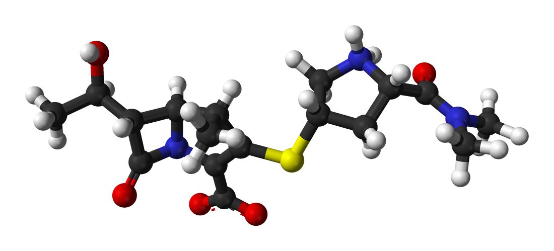
Above shows a diagram of the molecular structure of Meropenem [12]
However, since the model does not allow for the product to identify resistance to the last line of defence, requiring a later line of defence, we included colistin as the last treatment. Colistin has been used to treat multi-resistant NBM [14], however it is infrequently used due to its harmful side-effects [15].
The parameters of the model have hence been adjusted as such:
NBM has three lines of treatment: amoxicillin + cefotaxime/ceftriaxone, meropenem, and finally colistin. Therefore the model has three levels of treatment and corresponding resistance levels. The first level of treatment will henceforth be referred to as “Amoxicillin+” for the sake of conciseness.
There is a 100% mortality rate of untreated NBM [16]. Hence, we have set the chance of recovery if the pathogen is resistant to the current antibiotic in use to zero.
There is a 40% overall mortality rate in developed countries [16]. Therefore the parameters have been adjusted such that the expected outcome when our product is not in use averages to a 40% mortality rate.
Method
The parameters used in the model were as follows:
NUM_TIMESTEPS = 150
POPULATION_SIZE = 5000
INITIALLY_INFECTED = 50

DRUG_NAMES = ["Amoxicillin+", "Meropenem", "Colistin"]

PROBABILITY_MOVE_UP_TREATMENT = 0.2
TIMESTEPS_MOVE_UP_LAG_TIME = 5
ISOLATION_THRESHOLD = DRUG_NAMES.index("Colistin")

PRODUCT_IN_USE = True
PROBABILIY_PRODUCT_DETECT = 1
PRODUCT_DETECTION_LEVEL = DRUG_NAMES.index("Meropenem")

PROBABILITY_GENERAL_RECOVERY = 0
PROBABILITY_TREATMENT_RECOVERY = 0.3
PROBABILITY_MUTATION = 0.25
PROBABILITY_DEATH = 0.02
# Add time infected into consideration for death chance
DEATH_FUNCTION = lambda p, t: round(min(0.001*t + p, 1), 4)
PROBABILITY_SPREAD = 0.25
NUM_SPREAD_TO = 1
We ran the programme 10 times with the product in use and 10 times without. Albeit unrealistic in a hospital scenario, the population size was set to 5000 to minimise fluctuations between outcomes due to the stochastic nature of the model.
To further minimise the fluctuations, we then combined all the runs with and without the product respectively to create averaged runs. This meant that, for example, the deaths at timestep 20 of the averaged run without the product was the average of deaths at timestep 20 of each run when the product was not in use. If we had employed a deterministic model, these fluctuations would not be present, but we determined that the model was excessively complex to express as a deterministic model.
After each run we also calculated the Death rate (deaths as % of the population), the Mortality rate (deaths as % of the population that was infected), and the Infection rate (the population that was infected as % of the total population). We then calculated the sample mean and sample variance of the Death, Mortality and Infection rates of the runs with and without the product in use respectively. To confirm that there were statistically significant improvements in outcomes when using the product compared to not using the product, we conducted three one-sided hypothesis tests at the 1% level.
Since we used an unrealistically large population size in our initial runs, we also ran the programme again but with the parameters:
POPULATION_SIZE = 200
INITIALLY_INFECTED = 10
The graphic results of the runs with and without the product in use respectively were then compared to the averaged runs with populations of 5000. This confirmed that the population size does not adversely affect the results of the model, instead merely “smoothing the curve”, as Markov models with small sample sets tend to give very noisy data, given the law of large numbers.
Finally, we also did some further analysis into how the product affects the outcome of the model by looking a bit closer at the data. This involved looking at the change over time of cases of resistant pathogens and patients put into isolation.
Results and analysis
Outputs
In order to get a stronger understanding of the model, and prove that our product is helpful, we analysed the results of the model running in various scenarios.

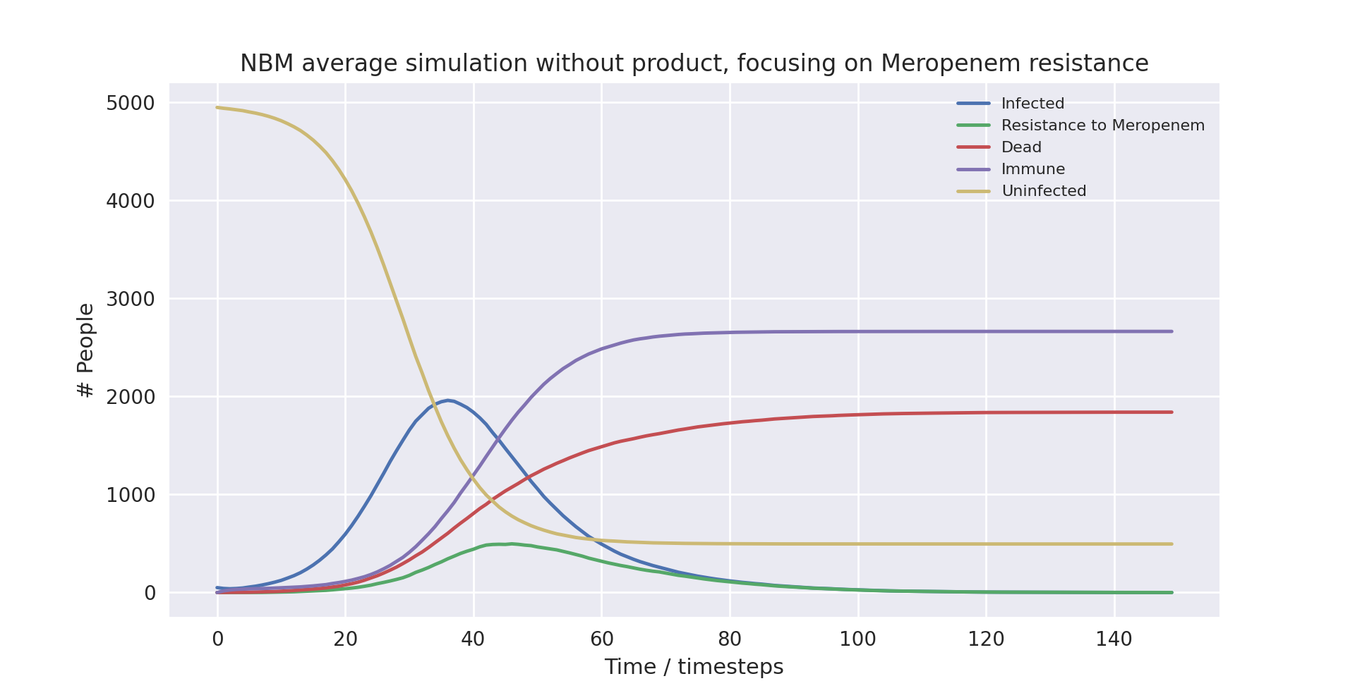
Above is a graph showing the change of several variables over time, having averaged 10 runs without the product in use. “Amoxicillin+”, “Meropenem”, and “Colistin” refer to the number of patients carrying a pathogen with resistance to said antibiotic(s). “Infected” is virtually indistinguishable from “Amoxicillin+” as almost all infected patients develop resistance to Amoxicillin+ immediately as treatment starts due to the parameters of the model. Only the first 100 time-steps are shown as the variables change only marginally after that.
Below are some statistics from the averaged run over a population of 5000 without the product in use:
Category |
Mean value |
Variance |
|---|---|---|
Number of deaths |
1840.6 |
2288 |
Number of infected people |
4504.9 |
653 |
Infection rate |
90.10% |
0.0026% |
Mortality rate |
40.86% |
0.0087% |
Death rate |
36.81% |
0.0093% |
The mortality rate of the averaged run without the product at 40.86% is very close to the actual mortality rate of NBM in developed countries. This means we have anchored the outcome correctly, which should give us more interesting takeaways when we compare with the outcome when the product is in use. The infection rate is very high, which is largely due to the model not simulating space (for example between departments of a hospital). Without a spatial element, there is no barrier to infection apart from people turning immune, dying or being put into isolation.

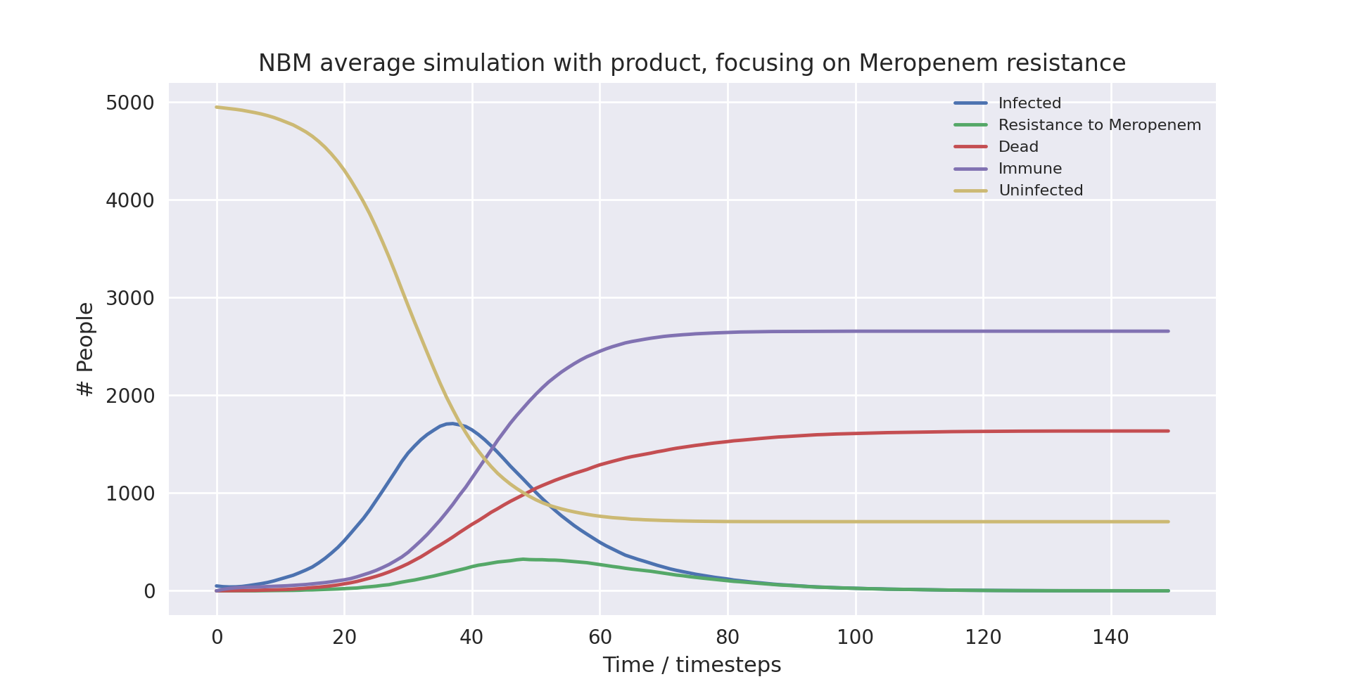
Above is a graph showing the change of several variables over time, having averaged 10 runs with the product in use. “Amoxicillin+”, “Meropenem”, and “Colistin” refer to the number of patients carrying a pathogen with resistance to said antibiotic(s). “Infected” is virtually indistinguishable from “Amoxicillin+” as almost all infected patients develop resistance to Amoxicillin+ immediately as treatment starts due to the parameters of the model. “Meropenem” is virtually indistinguishable from “Isolated” as all patients with resistance to Meropenem are put into isolation when the product is in use, with few patients being put into isolation that are not resistant to Meropenem. Only the first 100 time-steps are shown as the variables change only marginally after that.
Below are some statistics from the averaged run over a population of 5000 without the product in use:
Category |
Mean value |
Variance |
|---|---|---|
Number of deaths |
1635.8 |
270 |
Number of infected people |
4292.7 |
823 |
Infection rate |
85.85% |
0.0033% |
Mortality rate |
38.12% |
0.0013% |
Death rate |
32.73% |
0.0011% |
There is a clear difference in the number of mean deaths and mean infected compared to when the product was not in use. The total number of infections has dropped by 4.71% and the chance of dying among the infected (the mortality rate) has dropped by 6.56%. This results in a drop of total deaths by 11.13%, a notable improvement thanks to the product.
The drop in infection rates is because of the product proactively putting patients carrying a pathogen resistant to Meropenem in isolation. With more people put into isolation and patients on average being put into isolation earlier, infection rates will inevitably fall (this is covered in more detail in the ‘Further Analysis’ section). Importantly, the product does not only make use of isolation more often, it also ensures the right patients are isolated. The marginal increase in patients in isolation compared to when not using the product will all be from Meropenem-resistant or Colistin-resistant patients. Therefore, lower infection rates not only reflect an overall decrease in the spread of the disease, but they also reflect a decreased likelihood of a patient contracting a multidrug-resistant pathogen. This means the average patient with NBM is more likely to receive effective treatment, further causing mortality rates to drop.
The drop in mortality is therefore due to two reasons. The first is that, as we just outlined, a patient is less likely to carry a multidrug-resistant pathogen and is hence more likely to be treated effectively. The second is that once resistance to Meropenem has been detected, treatment immediately changes to Colistin. This means patients are not unnecessarily treated with Meropenem when it is not effective, decreasing their overall chance of dying.
Since the outcome of the model is largely dependent on probability, we must, however, before moving on verify that the product has led to the improved outcomes, rather than being a result of “fortuitous fluctuations”. In other words, we need to test whether these improvements are actually statistically significant.
Hypothesis tests
We conducted three difference-in-means hypothesis tests to verify that the product improved the outcomes of the runs. We compared the mean values of infection, mortality and death rates to ensure all improvements were statistically significant.
The null hypothesis is the initial presumption that the two mean values we are comparing are in fact equal and are part of the same distribution. To verify that our product has improved the average outcome, we must try to reject the null hypothesis. We reject the null hypothesis if the probability of a type I error is lower than the significance level chosen.
The probability of a type I error is the likelihood that you reject the null hypothesis when the null hypothesis is in fact correct. We chose a significance level of 1%, which means that if we are able to reject the null hypothesis, it is because there is a less than 1% chance that we are wrong.
While the purpose of our product was to decrease the overall number of deaths, we cannot know it has the intended effect on infection, mortality and death rates until we have tested it. Hence, we conducted two-sided hypothesis tests. This means that our alternative hypothesis (as opposed to the null hypothesis) was that the mean values for infection, mortality and death rates were either higher or lower when using the product than when not using it.
We can assume that the outcomes of the model follow a normal distribution. However, we do not know the standard deviation of outcomes. Therefore, we were left with two options: to approximate a normal distribution or to calculate the test based on a student’s t-distribution. Since we ran the simulations 10 times using and 10 times not using the product respectively, we have a sample size of 10 to calculate the mean values. This is a very low sample size, which suggested the most appropriate distribution was a student’s t-distribution. To know the degrees of freedom (DoF) of the t-test, we had to conduct F-tests of equality of variances test. The null hypothesis of these F-tests was that the variances were equal, while the two-sided alternative hypothesis was that they were not equal. For these tests we used a significance level of 10%.
To test equality of variances, we use this formula if \(S_1^2 > S_2^2\) :
And if \(S_1^2 < S_2^2\) , we use:
Where \(S_1^2\) is the sample variance of any given outcome variable when not using the product and \(S_2^2\) is the equivalent when using the product.
If we the find the variances to be equal, we calculate the probability of a Type I error using this formula:
With \(DoF=n_1+n_2-2\).
If we the find the variances to not be equal, we calculate the probability of a Type I error using the same formula but changing the degrees of freedom. With equal sample sizes we can calculate and simplify the degrees of freedom when variances are not equal as such:
We let \(\overline{x_1}\) be the mean value for any given outcome variable when not using the product and \(\overline{x_2}\) the mean value when using the product. \(n_1\) and \(n_2\) were the sample sizes, which was 10 in both cases. Since the initial assumption is that the null hypothesis holds, \(S_0^2\) is the hypothesised variance of the hypothesised real distribution, or in other words the square of the standard deviation of the hypothesised distribution.
Since the sample sizes are equal, we calculate the hypothesised variance using the formula:
Where \(S_1^2\) is the variance of any given outcome variable when not using the product and \(S_2^2\) is the equivalent when using the product.
Infection rates
For the equality of variances test of the infection rates, we used the following variables and calculation:
Category |
Value |
|---|---|
Variance of the infection rate without the product |
2.6\(\times 10^{-5}\) |
Variance of the infection rate with the product |
3.3\(\times 10^{-5}\) |
Hence, we do not reject the null hypothesis that the variances are equal. Therefore, the difference-in-means test of the infection rates was conducted using the following variables and calculation:
Category |
Value |
|---|---|
Mean infection rate without the product |
0.9010 |
Variance of the infection rate without the product |
2.6\(\times 10^{-5}\) |
Mean infection rate with the product |
0.8585 |
Variance of the infection rate with the product |
3.3\(\times 10^{-5}\) |
Hence, we reject the null hypothesis of no difference-in-means.
Mortality rates
For the equality of variances test of the mortality rates, we used the following variables and calculation:
Category |
Value |
|---|---|
Variance of the mortality rate without the product |
8.7\(\times 10^{-5}\) |
Variance of the mortality rate with the product |
1.3\(\times 10^{-5}\) |
Hence, we reject the null hypothesis that the variances are equal. Therefore, the difference-in-means test of the mortality rates was conducted using the following variables and calculation:
Category |
Value |
|---|---|
Mean infection rate without the product |
0.4086 |
Variance of the infection rate without the product |
8.7\(\times 10^{-5}\) |
Mean infection rate with the product |
0.3812 |
Variance of the infection rate with the product |
1.3\(\times 10^{-5}\) |
Hence, we reject the null hypothesis of no difference-in-means.
Death rates
For the equality of variances test of the mortality rates, we used the following variables and calculation:
Category |
Value |
|---|---|
Variance of the mortality rate without the product |
9.3\(\times 10^{-5}\) |
Variance of the mortality rate with the product |
1.1\(\times 10^{-5}\) |
Hence, we reject the null hypothesis that the variances are equal. Therefore, the difference-in-means test of the mortality rates was conducted using the following variables and calculation:
Category |
Value |
|---|---|
Mean infection rate without the product |
0.3682 |
Variance of the infection rate without the product |
9.3\(\times 10^{-5}\) |
Mean infection rate with the product |
0.3273 |
Variance of the infection rate with the product |
1.1\(\times 10^{-5}\) |
Hence, we reject the null hypothesis of no difference-in-means.
Thus, we see that all changes in means are statistically significant, implying that the product has significantly improved the expected outcome of the model.
Further analysis
Digging deeper into how the product impacts the outcome of the model, we can look at how variables interact over time. While the programme does not give us granular data to the extent that we can conditionalise the patients on certain variables, we can see how trends relate to each other.

Above is a graph showing the change of frequency in Meropenem and Colistin resistances as well as isolation over time, having averaged 10 runs without the product in use. As resistance to Colistin naturally yields resistance again Meropenem in the model, the frequency of resistance to Meropenem is always higher than that to Colistin. It is clear that isolation is lagging behind the spread of resistant pathogens, with many people who carry and could spread pathogens resistant to Meropenems not being put into isolation. At peak levels, resistance to Meropenem and Colistin reaches 496.8 and 256.5 respectively, while peak isolation reaches 295.5.

Above is a graph showing the change of frequency in Meropenem and Colistin resistances as well as isolation over time, having averaged 10 runs with the product in use. As resistance to Colistin naturally yields resistance again Meropenem in the model, the frequency of resistance to Meropenem is always higher than that to Colistin, however only by a slight amount. The frequency of resistance to Meropenem and that of being put into isolation is almost indistinguishable, as everyone who is resistant to Meropenem is put into isolation. The frequency of resistance to Meropenem is slightly higher than isolation levels while the disease is still spreading since patients only enter isolation the timestep after they develop Meropenem-resistance. At peak levels, resistance to Meropenem and Colistin reaches 323.6 and 271.7 respectively, while peak isolation reaches 313.5.
The first notable takeaway when comparing the data is the difference in frequency of resistance to Meropenem. At peak levels, not using the product increases the frequency of resistance to Meropenem by 53%. This is because patients who carry resistant pathogens are quickly put into isolation when using the product, preventing further spread. Notably, peak isolation is only 6% higher, which suggests that it is not merely putting more people into isolation that prevents spread.
Looking at timestep 30, isolation in the averaged run with the product is at 75.1, while isolation in the averaged run without the product is at 49.9, a massive 50.5% increase.
At timestep 60, isolation in the averaged run with the product is at 274.7, while isolation in the averaged run without the product is at 267.4, a mere 2.7% increase.
This rather qualitative look at the data suggests that the reason why the product prevents spread is not because it puts more people into isolation, but because it puts them into isolation earlier. This is important because it implies hospitals in the real world would not have to acquire higher capacity to accommodate patients with resistant pathogens, but can improve outcomes by using existing capacity more proactively.
Furthermore, the insights into isolation also explain why the product causes overall infection rates to decrease. While putting more people into isolation will inevitably decrease infection rates, putting them earlier into isolation will have the same effect.
Something else to note is the higher frequency of resistance to Colistin when using the product. Peak resistance when using the product reaches 271.7 compared to 256.5 when not using the product, a 5.9% increase. While this may not seem high, it has important implications as resistance again Colistin prevents the effective use of any antibiotic. Once a patient contracts a Colistin-resistant pathogen in this scenario, with no chance of a natural recovery, the patient is guaranteed to die.
Why does this happen? When the product detects resistance to Meropenem, treatment immediately changes to Colistin. This means that overall when using the product, more people are treated with Colistin than otherwise. Hence, while the frequency of Meropenem-resistance might be lower, the likelihood a pathogen develops resistance against Colistin if it is already resistant against Meropenem is much higher since resistance can only develop if it is treated with Colistin.
Is this a problem? Not necessarily, for two reasons. First of all, Colistin is only used when all other options are exhausted. In the case of a patient resistant to Meropenem, Colistin is the only effective treatment available to them. Since the chance of recovering without effective treatment is zero, not treating them is effectively letting them die. Furthermore, despite Colistin-resistance increasing in frequency, it is much less likely to spread. Without the product, we cannot know who carries Colistin-resistant pathogens, hence they are not guaranteed to be in isolation. Using the product, however, we always detect any patient resistant to Meropenem or any higher-tier antibiotic. This means all patients with resistance to Colistin are also put in isolation. Hence Colistin-resistance will not spread when the product is used. This is not totally true to the real world, and the change to fix this is discussed in the future work section, as we did not have time to propagate all the new data a fix to this would generate. However, we performed an informal test on the proposed fix (shown below), and found that the change appeared to be negligible.
if person.infection.get_tier() >= PRODUCT_DETECTION_LEVEL:
Is replaced by
if person.infection.get_tier() == PRODUCT_DETECTION_LEVEL:
Using a small population
Below, we show pairs of graphs of results with large and small population sizes for comparison
Above is a graph showing the change of several variables over time, taking the average of 10 runs without the product in use. “Meropenem” refers to the number of patients carrying a pathogen with resistance to Meropenem. Only the first 100 time-steps are shown as the variables change only marginally after that.
Above is a graph showing the change of several variables over time, when the population size was set to 200 and initially infected at 10, taking the average of 10 runs without the product in use. “Meropenem” refers to the number of patients carrying a pathogen with resistance to Meropenem. Only the first 100 time-steps are shown as the variables change only marginally after that.

Above is a graph showing the change of several variables over time, taking the average of 10 runs with the product in use. “Meropenem” refers to the number of patients carrying a pathogen with resistance to Meropenem. Only the first 100 time-steps are shown as the variables change only marginally after that.

Above is a graph showing the change of several variables over time, when the population size was set to 200 and initially infected at 10, taking the average of with the product in use. “Meropenem” refers to the number of patients carrying a pathogen with resistance to Meropenem. Only the first 100 time-steps are shown as the variables change only marginally after that.
As you can see, the runs with lower populations sizes and fewer infected at the start provide similar results to the averaged runs with much higher populations. They largely have the same outcomes, with the simulation not using the product ending up with 88%, 37% and 32% infection, mortality and death rates respectively, and the simulation using the product ending up with 90%, 35% and 32% infection, mortality and death rates respectively.
There are a few things worth noting. At surface level it seems as if the product made no difference in the runs with smaller population sizes, as the death rate was the same when using compared to when not using the product. Furthermore, in the run with the small population and with the product in use, the peak in cases was much earlier. The takeaway is that due to the model being stochastic, small sample sizes result in very different outcomes. This does not mean the product is less useful, it only points to the necessity of modelling with large enough sample sizes to get an accurate measurement of its impact.
All in all, the major trends seen in the simulations are very similar when comparing the averaged runs and the runs with the smaller populations. This indicates that the averaged runs give us a useful indicator of how the model works even with smaller populations.
Implications
Through our analysis we have been able to find several useful takeaways. First of all, in the case of neonatal bacterial meningitis, the product can decrease the total amount of deaths in a population through two means.
Ensuring patients carrying a pathogen resistant to Meropenem are treated with an effective treatment, such as Colistin, thereby lowering mortality rates.
Ensuring patients carrying a pathogen resistant to Meropenem are proactively put into isolation, directly lowering infection rates and indirectly lowering mortality rates, by preventing spread of Meropenem-resistance. Notably, the product does not seem to increase overall isolation rates by much. Rather, it puts patients into isolation earlier. Therefore hospitals are not required to increase isolation capacity, the product just allows any existing capacity to be used more effectively.
These two mechanisms work to decrease the infection rate by 4.71% and the mortality rate by 6.56%, overall resulting in a 11.13% lower death rate. Hypothesis testing confirmed all these improvements are statistically significant.
One cause for concern is the increased frequency of resistance to Colistin. At peak levels, using the product increased Colistin resistance by 5.9%. This is due to the product putting more people on Colistin treatment. While at surface level this might seem like an issue, one has to keep in mind two things.
The reason for higher use of Colistin is because all other options are exhausted. In the case of NBM, not treating a patient resistant to Meropenem with Colistin is effectively letting them die.
Thanks to the product putting patients resistant to Meropenem or any higher tier antibiotic in isolation, all patients with resistance to Colistin are also put in isolation. Hence Colistin-resistance will not spread.
While these statistics paint a promising picture, one needs to keep in mind that these are based on averaged runs with a large sample size. Were you to run the programme again trying to simulate the spread of NBM in an actual hospital department, the population will have to be decreased. Instead of using 5000 patients, a more realistic scenario would be hundreds or even tens of patients. Since the model is stochastic, the probabilities of individual events will lead to very different outcomes every time the programme is ran. Therefore, it is unrealistic to always expect the product to have the same impact. However, the test runs with populations of 200 tell us something interesting. While the outcomes will vary a lot, the averaged runs are good at predicting overall trends in terms of resistance frequencies and infection, mortality and death rates. Furthermore, they allow us to estimate the average impact of the product. Therefore, the unrealistic large population size of the averaged runs is not a reason to dispute any insights we get from them.
More generally, the contextualisation shows that the model can be useful to simulate real-world scenarios, and both qualify and quantify the impact of using the product. Generally, the more parameters that can be anchored, the more realistic the simulation and the more takeaways can be made. The simulation of our product being used to combat neonatal bacterial meningitis could just as well be applied to scenarios with other diseases, helping us understand how our product could make a difference there as well.
Development and future work
Throughout the development process, we presented the modelling work to other members of our team and our principal investigators, along with a mathematical biologist in the field, Alex Darlington. Presenting our work was helpful not only for ensuring that we could explain everything fully and understandably, but also as we received useful suggestions about ways we could improve the model.
A table of suggested improvements we received during development is:
Proposer |
Summary |
Used in final model? |
|---|---|---|
Alex Darlington |
Real hospitals only contain a fairly small number of people susceptible within the model, maximum 250, so the population size should be limited by that. This has the effect of increasing variance in the Markov model, as the law of large numbers does not apply, however, it is important for realistic simulation |
Yes |
Alex Darlington |
Add the use of a “last resort” drug, such as Colistin, to resolve the issue of the product detection being too late to make any meaningful action. For example, if a Carbapen is the final drug in the hierarchy, detection of resistance is not useful, as the highest possible isolation threshold is being treated with it, which is a pre-requisite for developing resistance, so people will never be isolated as a result, and there is no higher tier treatment to use, so better treatment cannot be given either. |
Yes |
Alex Darlington |
Add an increasing risk of death if a person has been infected for a long time, as in the real world, people become frail after having been sick for some time. |
Yes |
Axel Schoerner Emillon |
Change the detection method to only detect whether someone is currently resistant to Carbapenems, rather than if they have any higher tier resistance, as it is not a pre-requisite in the real world given that mutations might not occur in the Carbapenem treatment stage. This was not implemented as it was identified very late in the process after most of the analysis was completed and we would not have had time to redo it, but we performed an informal test, and found it caused a negligible difference in the model results. |
No |
A table of suggested future work we received during development is:
Proposer |
Summary |
Beneficial for future work? |
|---|---|---|
Alex Darlington |
Add a cap of the people who can be isolated at one time, as there is a physical limitation of beds in hospital. This was rejected as a change as isolation can be modelled as just more regular changing of PPE, rather than necessarily having totally discrete rooms. |
No |
Alex Darlington |
Add a spatial aspect to the model, for example having two wards which cannot spread to each other, but having staff who serve both wards and can become infected, in order to act as transmission vectors between the two wards. |
Yes |
Axel Schoerner Emillon |
Add an asymptomatic phase to the infections, where people can have the infection and be able to transmit it, but they are have no symptoms, so treatment will no start. |
Yes |
Conclusion
Given the fact that we have tested and validated our model to be sufficiently representative of the real world, and the model output indicates that the use of the product reduces the presence of antibiotic resistant pathogenic strains in our selected scenario, we conclude that our product is beneficial.
There are a number of aspects in which we could expand our model into if we did not have the time constraints of the iGEM competition, but we believe that the model in its current state both achieves its goal of showing our product is beneficial, along with being a useful tool for understanding the issue of antibiotic resistance in its own right.
Discussion
Some common questions about the model are answered below:
Is the model realistic?
A. The model is a balance of realism with abstraction. If the model were designed to be holly realistic model, it would inevitably turn into a “hospital simulator”, would be too complex to design, and take too long to run on current computers. However, the model must not be too heavily abstracted, as otherwise it does not fully encode the complexities of the system. We carefully designed the model to only consider the aspects of the real world we thought relevant to its results, and abstracted away the rest, and were shown to have done this correctly by completing the validation process. In summary, the model is realistic “where it counts”, but it does not simulate unnecessary complexities
Is the model useful?
Yes, because it provides several helpful insights:
The impact our product will have on the spread of resistance just by quickly detecting who to put into isolation
Whether higher or lower mortality or transmissibility of a disease increase or decrease the effectiveness
What potential improvements are there?
A. It would be possible to add additional features to the model to make it more realistic, for example:
Spatial considerations – e.g. modelling multiple wards with movement between them
Asymptomatic transmission periods of infection
however, these are beyond the scope of our project
How does the model compare to other existent ones?
A. Our model is designed specifically for modelling the development of antibiotic resistance in a population. The techniques and type of model we employed are fairly common in the field of modelling pathogens, as they work particularly well! However, our model differs in several ways. Firstly, it includes the major feature of differentiating between whether our product is in use, which is a feature in no other published models, as our product is novel. Secondly, most academic publications only include results, whereas we openly include the model code at the fore-front of our research, and encourage people to use and build off our code. With this in mind, we designed it to be readable, and provided clear documentation for all its features.
Why not use a deterministic model?
A. The complexity of the logic in the model is very high, so it would be exceedingly difficult to design a system of equations to form the deterministic model that defines it. The benefit of stochastic models is that they can be expressed declaratively rather than imperatively - i.e. only the properties, rather than a full definition of the system need be given. This makes it easier to both develop and validate the model. The drawback of stochastic models is that for small populations they can produce noisy data. However, since we showed that population size doesn’t affect the model results, and we averaged the model results over many (at least 10, dependent on scenario) number of runs, the noise was negligible.
Q. Can the model be applied to current issues, i.e. the COVID pandemic?
A. Since the model is a very generic abstraction of the real world, by adjusting it’s parameters a vast amount of different scenarios can be modelled. The key issue in adapting it to different scenarios is if they fit the inherent logic and states hard-coded into it. Since COVID is a viral infection, as opposed to a bacterial infection, antibiotics cannot be used to treat it, so the tiered system of antibiotic uses fits less cleanly to it, however, they could instead be considered as increasingly aggressive treatment options, to which it also grows resistant. However, the logic around our product would not apply, as viral infections are not affected by carbapenem, which is the antibiotic we focus on.
References
[1] Kermack, W O. McKendrick, A G. 1927. A contribution to the mathematical theory of epidemics. Proc. R. Soc. Lond. A 115: 700–721 http://doi.org/10.1098/rspa.1927.0118
[2] Simon, C., 2020. The SIR dynamic model of infectious disease transmission and its analogy with chemical kinetics. PeerJ Physical Chemistry, 2, p.e14.
[3] Niewiadomska, A. Jayabalasingham, B. Seidman, J. Willem, L. Grenfell, B. Spiro, D. Viboud, C. 2019. Population-level mathematical modeling of antimicrobial resistance: a systematic review. BMC Medicine. Available at: https://bmcmedicine.biomedcentral.com/articles/10.1186/s12916-019-1314-9 [Accessed 16 October 2021]
[4] Lakin, S. Kuhnle, A. Alipanahi, B. Noyes, N. Dean, C. Muggli, M. Raymond, R. Abdo, Z. Prosperi, M. Belk, K. Morley, P. Boucher, C. 2019. Hierarchical Hidden Markov models enable accurate and diverse detection of antimicrobial resistance sequences. Nature. Available at: https://www.nature.com/articles/s42003-019-0545-9 [Accessed 16 October 2021]
[5] Love, W. Zawack, K. Booth, J. Grӧhn, Y. Lanzas, C. 2016. Markov Networks of Collateral Resistance: National Antimicrobial Resistance Monitoring System Surveillance Results from Escherichia coli Isolates, 2004-2012. PLOS Computational Biology. Available at: https://journals.plos.org/ploscompbiol/article?id=10.1371/journal.pcbi.1005160 [Accessed 16 October 2021]
[6] Murray-Smith, D. 2015. Testing and Validation of Computer Simulation Models: Principles, Methods and Applications (1st. ed.). Springer Publishing Company, Incorporated.
[7] Dubien, N. 2018, Introduction to Property Based Testing - Another test philosophy introduced by QuickCheck. Available at: https://medium.com/criteo-engineering/introduction-to-property-based-testing-f5236229d237 [Accessed 16 October 2021]
[8] Nygard, M. 2013. Better Than Unit Tests. Cognitect blog. Available at: https://www.cognitect.com/blog/2013/11/26/better-than-unit-tests [Accessed 16 October 2021]
[9] Kathleen, C. 1996. Validating Computational Models. [pdf] Available at: casos.cs.cmu.edu/publications/papers/howtoanalyze.pdf [Accessed 16 October 2021]
[10] Kleijnen, J. 1995. Statistical Validation of Simulation Models. European Journal of Operational Research, 82(1): 145-162
[11] Şah İpek, M., 2019. Neonatal Bacterial Meningitis. Neonatal Medicine.
[12] 2017. Management of Bacterial Meningitis in infants <3 months. [pdf] Meningitis Research Foundation. Available at: https://www.meningitis.org/getmedia/75ce0638-a815-4154-b504-b18c462320c8/Neo-Natal-Algorithm-Nov-2017 [Accessed 15 October 2021].
[13] Mills, B. 2009. Ball-and-stick model of the meropenem molecule. Wikimedia Commons. Available at: https://commons.wikimedia.org/wiki/File:Meropenem-from-xtal-1992-3D-balls.png [Accessed 19 October 2021]
[14] Mahabeer, P., Mzimela, B., Lawler, M., Singh-Moodley, A., Singh, R. and Mlisana, K., 2018. Colistin-resistant Acinetobacter baumanniias a cause of neonatal ventriculitis. Southern African Journal of Infectious Diseases, pp.1-3.
[15] Nation, R. and Li, J., 2009. Colistin in the 21st century. Current Opinion in Infectious Diseases, 22(6), pp.535-543.
[16] Tesini, B., 2020. Neonatal Bacterial Meningitis. [online] MSD Manual Professional Edition. Available at: https://www.msdmanuals.com/en-gb/professional/pediatrics/infections-in-neonates/neonatal-bacterial-meningitis [Accessed 15 October 2021].